Land use and land cover classification with multispectral Sentinel-2 satellite images and TensorFlow
In this post I will show how you obtain a ready-to-use training dataset with Sentinel-2 satellite images, train a CNN with TensorFlow and Keras and create a Land use and land cover map for new and unseen data.
TensorFlow Datasets is a collection of tf.data.Datasets that can be used without the hassle of manually downloading and preparing training data. EuroSat is a dataset of 27,000 labeled and geo-referenced images in 10 classes with 13 spectral bands. It is available as TensorFlow Dataset definition.
Loading the dataset
Here we use the all dataset configuration that contains all 13 image bands and not just RGB. We use 80% of the dataset for training, retain 10% as validation and another 10% for the final classifier assessment as test set.
import tensorflow as tf
import tensorflow_datasets as tfds

(ds_train, ds_valid, ds_test), ds_info = tfds.load('eurosat/all',
                                                   split=['train[:80%]','train[80%:90%]','train[90%:]'],
                                                   as_supervised=True,
                                                   with_info=True)
NUM_CLASSES = ds_info.features['label'].num_classes
CLASS_NAMES = ds_info.features['label'].names
print('number of samples in train, valid, test:',
      [tf.data.experimental.cardinality(ds).numpy() for ds in [ds_train,ds_valid,ds_test]])
print('class names:', CLASS_NAMES)

# > number of samples in train, valid, test: [21600, 2700, 2700]
# > class names: ['AnnualCrop', 'Forest', 'HerbaceousVegetation', 'Highway', 'Industrial', 'Pasture', 'PermanentCrop', 'Residential', 'River', 'SeaLake']
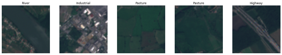
Inspecting the dataset
In the next step we want to visualize some samples as RGB images. The image bands are available as UInt16 “Digital Numbers” (DN) that need to be converted to reflectances by dividing them by 10,000. The reflectance has a typical range of [0.0, 0.4] but as the documentation states, higher values are expected in infrared bands. To normalize the reflectance values we simply multiply them by 2.5 and clip them to the [0.0, 1.0] range to properly display them:
import matplotlib.pyplot as plt
import numpy as np

DN = 10_000

def normalize(tensor):
    tensor /= DN
    tensor *= 2.5
    return tf.clip_by_value(tensor, 0., 1.)

def ms_to_rgb(tensor):
    band_r = tensor[..., 3]
    band_g = tensor[..., 2]
    band_b = tensor[..., 1]
    return normalize(tf.stack([band_r, band_g, band_b], axis=-1))

def show_rgb_samples(ds):
    number_samples = tf.data.experimental.cardinality(ds).numpy()
    fig, axs = plt.subplots(1, number_samples, figsize=(number_samples * 5, 5), squeeze=False)
    for index, (tensor, label) in enumerate(ds):
        if tf.rank(label) == 0:
            title = CLASS_NAMES[label.numpy()]

        else: #label is a tensor with probabilities
            title = f'{CLASS_NAMES[tf.math.argmax(label)]} ({tf.math.reduce_max(label):.3f})'

        axs[0, index].imshow(ms_to_rgb(tensor))
        axs[0, index].set_title(title)
        axs[0, index].axis('off')

show_rgb_samples(ds_train.take(5))
Training
For training we use a custom function to standardize each sample. We calculated the mean and standard deviation for each band in the training set. Each sample in the train, validation and test datasets gets standardized by subtracting the mean and dividing the standard deviation per band. We also want to augment our train dataset and randomly flip and rotate each sample.
import tensorflow_addons as tfa

MEANS = [1353.4839, 1117.0938, 1042.1034, 946.73224, 1199.5142, 2005.943, 2378.6394, 2305.6174, 732.0749, 12.07309,
         1822.308, 1118.718, 2605.0498]
STDDEVS = [65.17162, 153.58511, 187.4783, 277.7896, 227.93288, 356.2915, 455.57788, 531.0652, 98.77772, 1.1824766,
           378.07095, 302.88586, 502.6844]

@tf.function
def standardize(tensor, *args):
    band_tensors=[]
    for c in range(tensor.shape[-1]):
        t = tf.cast(tensor[..., c], tf.float32)
        t -= MEANS[c]
        t /= STDDEVS[c]
        band_tensors.append(t)
    tensor= tf.stack(band_tensors, -1)
    return (tensor, tf.one_hot(args[0], NUM_CLASSES)) if len(args) == 1 else tensor

@tf.function
def augment(tensor, label):
    angle = tf.random.uniform(shape=[], minval=-180, maxval=180, dtype=tf.float32)
    tensor = tfa.image.rotate(tensor, angle)
    tensor = tf.image.random_flip_left_right(tensor)
    return tensor, label

BATCH_SIZE = 32
BUFFER_SIZE = tf.data.experimental.cardinality(ds_train).numpy()

ds_train = ds_train\
    .map(standardize, num_parallel_calls=tf.data.experimental.AUTOTUNE)\
    .cache()\
    .map(augment, num_parallel_calls=tf.data.experimental.AUTOTUNE)\
    .shuffle(BUFFER_SIZE)\
    .batch(BATCH_SIZE)\
    .prefetch(tf.data.experimental.AUTOTUNE)

ds_valid = ds_valid\
    .map(standardize, num_parallel_calls=tf.data.experimental.AUTOTUNE)\
    .cache()\
    .batch(BATCH_SIZE)\
    .prefetch(tf.data.experimental.AUTOTUNE)

ds_test = ds_test\
    .map(standardize, num_parallel_calls=tf.data.experimental.AUTOTUNE)\
    .batch(BATCH_SIZE)
We train a DenseNet-121 model from scratch with an initial learning rate of 1e-4 and a batch size of 32 for 100 epochs. We also apply an early stopping callback that stops the training if the validation loss hasn’t improved for seven epochs and a reduce learning rate callback that reduces the metric if the validation loss hasn’t improved for four epochs. Once the training is finished we evaluate our model on the test dataset.
import os

out_dir='out'
METRICS = [tf.keras.metrics.CategoricalAccuracy(name='accuracy'),
           tf.keras.metrics.Precision(),
           tf.keras.metrics.Recall()]

model = tf.keras.applications.densenet.DenseNet121(include_top=True, weights=None, input_tensor=None, input_shape=(64,64,13), pooling=None, classes=NUM_CLASSES)
model.compile(optimizer=tf.keras.optimizers.Adam(learning_rate=1e-4), loss='categorical_crossentropy', metrics=METRICS)

early_stopping_callback = tf.keras.callbacks.EarlyStopping(monitor='val_loss', patience=7, restore_best_weights=True)
reduce_lr_callback = tf.keras.callbacks.ReduceLROnPlateau(monitor='val_loss', factor=0.1, patience=4)
callbacks = [early_stopping_callback, reduce_lr_callback]

model.fit(ds_train,
          epochs=100,
          validation_data=ds_valid,
          callbacks=callbacks)
model.save(os.path.join(out_dir, 'model'))
model.evaluate(ds_test)

# > [...]
# > Epoch 46/100
# > 675/675 [==============================] - 60s 64ms/step - loss: 0.0179 - accuracy: 0.9937 - precision: 0.9944 - recall: 0.9935 - val_loss: 0.0562 - val_accuracy: 0.9837 - val_precision: 0.9837 - val_recall: 0.9826
# > INFO:tensorflow:Assets written to: out/model/assets
# > 85/85 [==============================] - 4s 39ms/step - loss: 0.0567 - accuracy: 0.9841 - precision: 0.9855 - recall: 0.9830
In the above run, the model training was stopped after 46 epochs and we achieved a top-1 accuracy of 0.9841 on the unseen test set which is on par with the numbers from the EuroSat paper.
Classification of new samples
In the next step we want to classify a completely new scene. You can download new images either on the Copernicus Open Access Hub or the Sentinel Hub EO Browser. In both cases you need to register first. I recommend using the Level-1C (top-of-atmosphere) products as the Level-2A (bottom-of-atmosphere) products are preprocessed and missing some redundant bands.
Important to note is the band order the EuroSat dataset was created with. The last band is 8A, not 12:
| Band index in dataset |
Sentinel-2 band | Resolution (m) |
Central wavelength (nm) |
|---|---|---|---|
| 0 | Band 1 - Coastal aerosol | 60 | 443 |
| 1 | Band 2 - Blue | 10 | 490 |
| 2 | Band 3 - Green | 10 | 560 |
| 3 | Band 4 - Red | 10 | 665 |
| 4 | Band 5 - Vegetation red edge 1 | 20 | 705 |
| 5 | Band 6 - Vegetation red edge 2 | 20 | 740 |
| 6 | Band 7 - Vegetation red edge 3 | 20 | 783 |
| 7 | Band 8 - NIR | 10 | 842 |
| 8 | Band 9 - Water vapour | 60 | 945 |
| 9 | Band 10 - SWIR - Cirrus | 60 | 1375 |
| 10 | Band 11 - SWIR 1 | 20 | 1610 |
| 11 | Band 12 - SWIR 2 | 20 | 2190 |
| 12 | Band 8A - Narrow NIR | 20 | 865 |
When you download the Level-1C data from the sources above you get a ZIP archive that contains all image bands as separate jp2 files. The next step is to create a single image tensor of shape (img_height, img_width, 13) from the individual image files and upsample the bands with a resolution of 20m or 60m to 10m:
import cv2
from tqdm import tqdm

def jp2_to_tensor(path_template):
    band_resolution = [('B01', 60), ('B02', 10), ('B03', 10), ('B04', 10), ('B05', 20), ('B06', 20), ('B07', 20),
                       ('B08', 10), ('B09', 60), ('B10', 60), ('B11', 20), ('B12', 20), ('B8A', 20),]

    band_images = []
    for band, resolution in tqdm(band_resolution):
        path = path_template.format(band)
        band_image = cv2.imread(path, cv2.IMREAD_UNCHANGED)

        factor = resolution/10.
        band_image = cv2.resize(band_image, (0,0), fx=factor, fy=factor, interpolation=cv2.INTER_NEAREST)
        band_images.append(tf.convert_to_tensor(band_image))
    return tf.stack(band_images, axis=-1)

sample = jp2_to_tensor('./S2A_MSIL1C_20211203T095401_N0301_R079_T33UXQ_20211203T105856.SAFE/GRANULE/L1C_T33UXQ_A033681_20211203T095357/IMG_DATA/T33UXQ_20211203T095401_{}.jp2')
print(sample.shape)

# > 100%|██████████| 13/13 [01:44<00:00,  8.08s/it]
# > (10980, 10980, 13)
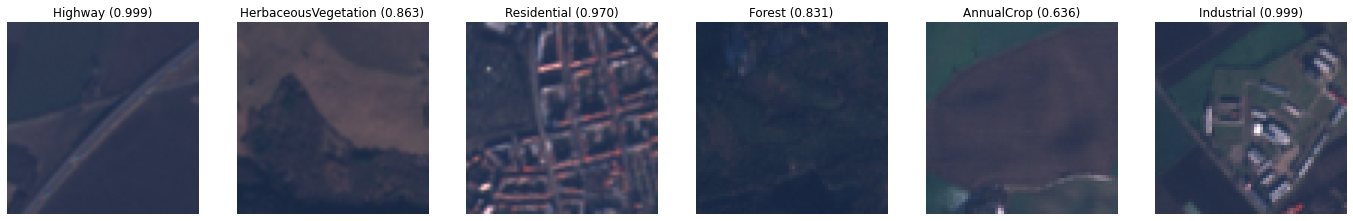
As the model was trained on 64 x 64 px image patches, we want to predict patches of the same dimensions from that sample and output the probability for the top-1 class:
PATCH_HW = 64
sample_offsets=((6208, 1409), (9576, 7376), (4871, 1580), (4981, 10360), (4794, 4500), (7432, 7950))
sample_tensors = [sample[row:row + PATCH_HW, column:column + PATCH_HW, :] for row, column in sample_offsets]
sample_tensors = tf.stack(sample_tensors, axis=0)

raw_predictions = model.predict(standardize(sample_tensors))
ds_prediction = tf.data.Dataset.from_tensor_slices((sample_tensors, raw_predictions))
show_rgb_samples(ds_prediction)
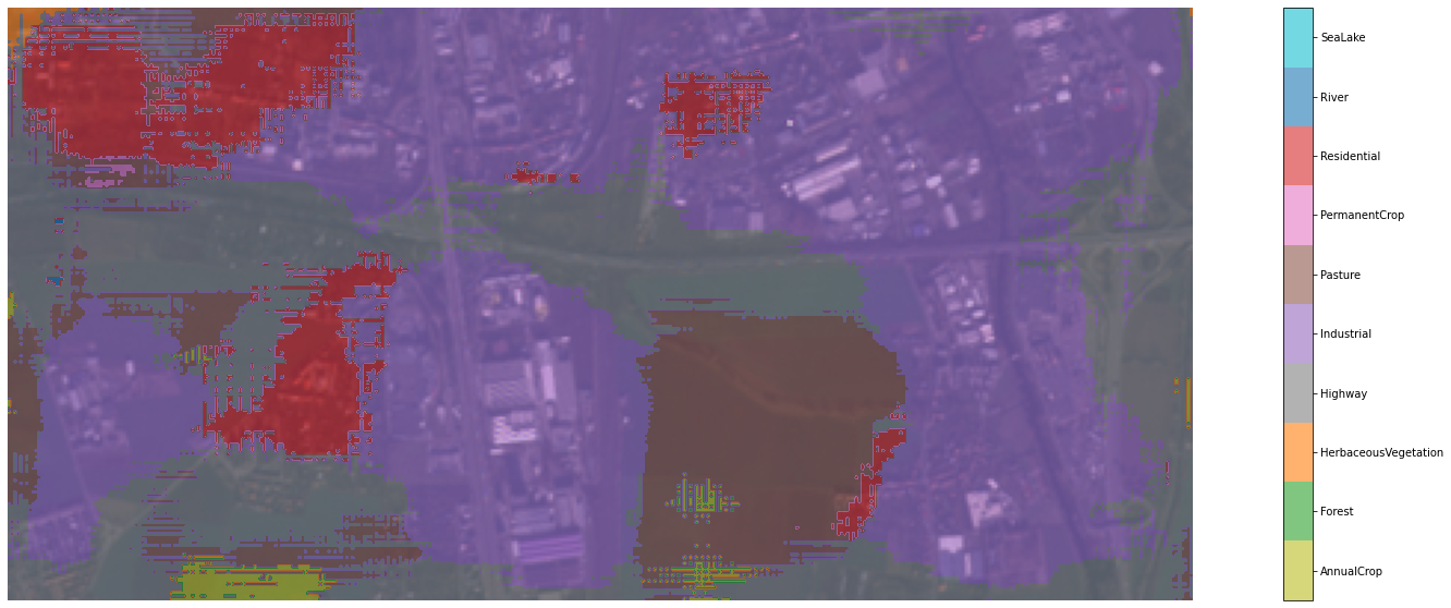
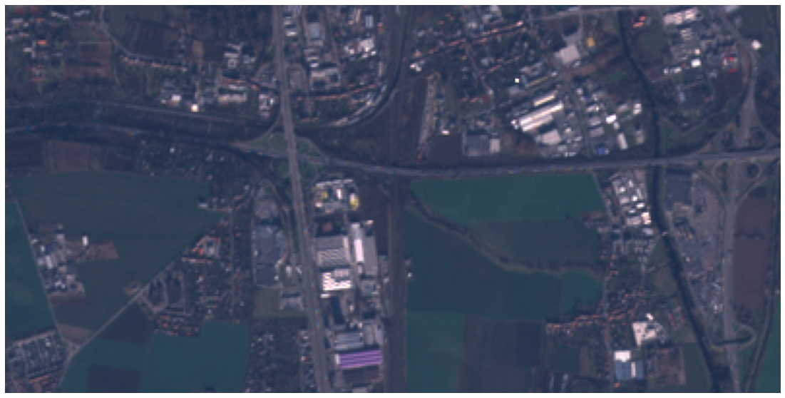
In the next step we want to predict a larger scene from the original sample image and plot a classification mask on top of it.
h, w = 200, 400
offset_h, offset_w = 5278, 1514

scene_raw = sample[offset_h:offset_h+h, offset_w:offset_w+w, :]
scene_height, scene_width, scene_num_bands = scene_raw.shape

plt.figure(figsize=(10,5))
plt.imshow(ms_to_rgb(scene_raw))
plt.axis('off')
plt.show()

scene = standardize(scene_raw)
scene = tf.expand_dims(scene, 0)
From the scene above we create a dataset of 64x64 patches with the help of tf.image.extract_patches. This collects patches from the image as if applying the convolution operation. The SAME padding flag creates a padding of zeroes around a patch for areas outside of the input. With that approach we classify each pixel of the scene.
patches = tf.image.extract_patches(scene, [1, PATCH_HW, PATCH_HW, 1], [1,1,1,1], [1,1,1,1], 'SAME')
patches = tf.reshape(patches, [patches.shape[-2] * patches.shape[-3], PATCH_HW, PATCH_HW, scene_num_bands])
patches_dataset = tf.data.Dataset.from_tensor_slices(patches)
preds = model.predict(patches_dataset.batch(32), verbose=1)
preds_top_1 = np.argmax(preds, axis=-1)
preds_top_1 = np.reshape(preds_top_1, (scene_height, scene_width))

# > 2500/2500 [==============================] - 738s 263ms/step
Finally, we want to display our classification mask on top of our scene image. This is possible with the help of some Matplotlib magic. The result you can see at the top of this post.
from matplotlib.colors import ListedColormap, BoundaryNorm
from matplotlib.ticker import FuncFormatter

color_dict = {
    0: 'tab:olive', #AnnualCrop
    1: 'tab:green', #Forest
    2: 'tab:orange', #HerbaceousVegetation
    3: 'tab:gray', #Highway
    4: 'tab:purple', #Industrial
    5: 'tab:brown', #Pasture
    6: 'tab:pink', #PermanentCrop
    7: 'tab:red', #Residential
    8: 'tab:blue', #River
    9: 'tab:cyan', #SeaLake
}

cm = matplotlib.colors.ListedColormap([color_dict[x] for x in color_dict.keys()])

labels = np.array(CLASS_NAMES)
len_lab = len(labels)

norm_bins = np.sort([*color_dict.keys()]) + 0.5
norm_bins = np.insert(norm_bins, 0, np.min(norm_bins) - 1.0)

norm = BoundaryNorm(norm_bins, len_lab, clip=True)
fmt = FuncFormatter(lambda x, pos: labels[norm(x)])

fig,ax = plt.subplots(figsize=(30,10))
ax.axis('off')
ax.imshow(ms_to_rgb(scene_raw))
im = ax.imshow(preds_top_1, alpha=0.6, cmap=cm, norm=norm)

diff = norm_bins[1:] - norm_bins[:-1]
tickz = norm_bins[:-1] + diff / 2
cb = fig.colorbar(im, format=fmt, ticks=tickz)